47. The Kalman Filter and Vector Autoregressions#
47.1. Overview#
This lecture derives the Kalman filter for a linear Gaussian state space system and then uses it to construct vector autoregressions (VARs).
It builds on A First Look at the Kalman Filter, where the filter is introduced through filtering and forecasting distributions.
It complements Another Look at the Kalman Filter, where the same recursion is used in a worker-firm learning problem.
This lecture shifts attention from filtering a hidden state to representing and estimating the observable process generated by that hidden state.
Our approach rests on repeated applications of the population linear least squares projection formula, the insight that computing a conditional expectation of a jointly normal random vector is the same as running a population OLS regression.
The lecture covers:
deriving the Kalman filter recursions from first principles
the matrix Riccati difference equation governing conditional covariance matrices
the innovations representation and the Gram-Schmidt whitening property
the structure of a hidden Markov model
the likelihood function for a state space system and its role in maximum likelihood and Bayesian estimation
how the time-invariant Kalman filter generates a vector autoregression
why the Kalman filter is an essential tool for interpreting VARs estimated from economic data
47.2. The state space system#
The Kalman filter applies to the state space system for \(t \geq 0\):
where
\(x_t\) is an \(n \times 1\) state vector (hidden, unobserved)
\(y_t\) is an \(m \times 1\) vector of signals on the hidden state (observed)
\(w_{t+1}\) is a \(p \times 1\) IID sequence of normal random variables with mean \(0\) and identity covariance matrix
\(v_t\) is an IID sequence of normal random variables with mean zero and covariance matrix \(R\)
\(w_{t+1}\) and \(v_s\) are orthogonal for all \(t+1\) and \(s \geq 0\)
The coefficient matrices have the following dimensions: \(A\) is \(n \times n\), \(C\) is \(n \times p\), \(G\) is \(m \times n\), and \(R\) is \(m \times m\).
The initial state satisfies
We observe \(y_t, \ldots, y_0\) but not \(x_t, \ldots, x_0\) at time \(t\), and we know all first and second moments implied by (47.1) and (47.2).
47.3. The Kalman filter#
47.3.1. Starting distribution#
Working forward in time starting at \(t = 0\), before observing \(y_0\), the specification (47.1)-(47.2) implies that the marginal distribution of \(y_0\) is
For \(t \geq 0\) let \(y^t = [y_t, y_{t-1}, \ldots, y_0]\).
We want a convenient recursive representation of the conditional distribution of \(y_t\) given history \(y^{t-1}\).
The Kalman filter attains this by constructing recursive formulas for \(\hat{x}_t\) and \(\Sigma_t\) such that the distribution of \(y_t\) conditional on \(y^{t-1}\) generalises (47.3) to
for \(t \geq 1\), where the distribution of \(x_t\) conditional on \(y^{t-1}\) is \(N(\hat{x}_t, \Sigma_t)\).
The objects \(\hat{x}_t\) and \(\Sigma_t\) characterise the population regression
and the conditional covariance matrix
47.3.2. Derivation#
At each date, our approach is to regress what we do not know on what we know.
Note
Because our assumptions imply that \(\{x_t, y_t\}_{t=0}^\infty\) is a jointly normal stochastic process, linear least squares regressions equal conditional mathematical expectations.
Each step below is an application of Bayes’ law.
Under the weaker assumption that all means and covariances exist without joint normality, the same calculations yield “wide-sense conditional expectations” that coincide with true conditional expectations only when those conditional expectations are linear.
We arrive at \(t = 0\) knowing \(\hat{x}_0\) and \(\Sigma_0\).
The information about \(x_0\) in \(y_0\) that is new relative to \((\hat{x}_0, \Sigma_0)\) is the innovation
Let \(L_0\) be the population regression coefficient of the hidden-state error \(x_0-\hat{x}_0\) on the signal surprise \(y_0-G\hat{x}_0\).
The conditional mean \(\mathbb{E}[x_0 \mid y_0] = \hat{x}_0 + L_0(y_0 - G\hat{x}_0)\) satisfies the population regression formula
where \(\eta\) is the least squares residual.
Orthogonality of \(\eta\) to \((y_0 - G\hat{x}_0)\) pins down \(L_0\) via the normal equations
Evaluating the moment matrices and solving for \(L_0\) gives
Thus \(L_0\) updates the estimate of \(x_0\), while \(K_0=A L_0\) updates the forecast of \(x_1\).
To forecast \(x_1\), note that
Applying (47.5) gives \(\mathbb{E}[x_1 \mid y_0] = A\hat{x}_0 + AL_0(y_0 - G\hat{x}_0)\), which we write as
where the Kalman gain at time 0 is
Subtracting (47.8) from (47.7) yields
Using (47.10) and \(y_0 = G x_0 + v_0\) to evaluate \(\Sigma_1 \equiv \mathbb{E}[(x_1 - \hat{x}_1)(x_1 - \hat{x}_1)^\top \mid y_0]\) gives
Thus \(f(x_1 \mid y_0) \sim N(\hat{x}_1, \Sigma_1)\).
Collecting the time-\(0\) equations:
System (47.12) maps a mean-covariance pair \((\hat{x}_0, \Sigma_0)\) into a new pair \((\hat{x}_1, \Sigma_1)\), with auxiliary outputs \((a_0, K_0)\).
Recognising that “we are in the same situation at the start of period 1 as at the start of period 0” activates a recursion, the Kalman filter.
47.3.3. The Kalman filter recursions#
Iterating system (47.12) yields the Kalman filter for \(t \geq 0\):
Here \(K_t\) is the Kalman gain at time \(t\).
47.3.4. The matrix Riccati equation#
Substituting the expression for \(K_t\) from the second line of (47.13) into the fourth line gives an equivalent update formula:
Equation (47.14) is the matrix Riccati difference equation.
It governs the sequence of conditional covariance matrices \(\{\Sigma_t\}_{t=0}^\infty\) without reference to the observations \(\{y_t\}\).
47.4. The Gram-Schmidt process#
The random vector
is the innovation of \(y_t\) with respect to \(y^{t-1}\), the part of \(y_t\) that cannot be predicted from past observations.
Note that \(\mathbb{E} a_t a_t^\top = G\Sigma_t G^\top + R\), the matrix whose inverse appears in the Kalman gain formula (47.13).
A direct calculation using \(a_t = G(x_t - \hat{x}_t) + v_t\) shows that \(\mathbb{E} a_t a_{t-1}^\top = 0\) and, more generally, \(\mathbb{E}[a_t \mid a_{t-1}, \ldots, a_0] = 0\).
Note
An alternative argument from first principles: let \(H(y^t)\) denote the closed linear span of \(y^t\).
Since \(a_{t+1} = y_{t+1} - \mathbb{E}[y_{t+1} \mid y^t]\) is a least-squares error, \(a_{t+1} \perp H(y^t)\), and in particular \(a_{t+1} \perp a_t\).
Thus \(\{a_t\}\) is a white-noise process of innovations to \(\{y_t\}\).
Sometimes (47.13) is called a whitening filter: it takes the signal process \(\{y_t\}\) as input and produces the white-noise innovation process \(\{a_t\}\) as output.
With \(H(a^t)\) defined analogously, the linear space \(H(a^t)\) is an orthogonal basis for the linear space \(H(y^t)\).
Rather than computing \(\mathbb{E}[x_t \mid y_{t-1}, \ldots, y_0]\) via one large regression, the Kalman filter performs a sequence of small regressions on successive orthogonal components of the basis \([a_{t-1}, \ldots, a_0]\), an instance of the Gram-Schmidt procedure.
47.6. Estimation#
47.6.1. The innovations representation#
The innovations representation emerging from the Kalman filter is
where \(\hat{x}_t = \mathbb{E}[x_t \mid y^{t-1}]\) for \(t \geq 1\) and \(\mathbb{E}[a_t a_t^\top \mid y^{t-1}] = G\Sigma_t G^\top + R \equiv \Omega_t\).
For \(t \geq 1\), \(\mathbb{E}[y_t \mid y^{t-1}] = G\hat{x}_t\) and the conditional distribution of \(y_t\) given \(y^{t-1}\) is \(N(G\hat{x}_t, \Omega_t)\).
The objects \((G\hat{x}_t, \Omega_t)\) emerging from the Kalman filter recursions therefore completely characterise this conditional distribution.
47.6.2. The likelihood function#
We can factor the likelihood of a sample \((y_T, y_{T-1}, \ldots, y_0)\) as
The log conditional density of the \(m \times 1\) vector \(y_t\) is
Using (47.17) and (47.13) together, we can evaluate the likelihood (47.16) recursively for any parameter vector \(\theta\) that underlies the matrices \(A, G, C, R\).
Such calculations are at the heart of efficient strategies for computing maximum likelihood estimators of free parameters.
47.6.3. Bayesian inference#
The likelihood function is also central to Bayesian inference.
Where \(\theta\) is the parameter vector, \(y_0^T\) the data, and \(\tilde{p}(\theta)\) a prior density over \(\theta\) before seeing \(y_0^T\), Bayes’ law gives the posterior
The denominator is the marginal joint density \(f(y_0^T)\).
47.7. Vector autoregressions and the Kalman filter#
47.7.1. Convergence to a steady state#
Under conditions discussed by Anderson et al. [1996], iterations on the Riccati equation (47.14) converge to a time-invariant matrix \(\Sigma\) from any positive semi-definite starting value \(\Sigma_0\).
A time-invariant fixed point \(\Sigma_t = \Sigma\) of (47.14) is the covariance matrix of \(x_t\) around
where the conditioning extends over the semi-infinite past \(s \leq t-1\).
47.7.2. A time-invariant VAR#
If the fixed point \(\Sigma\) exists and we initialise the filter at \(\Sigma_0 = \Sigma\), the innovations representation (47.15) becomes time-invariant:
where \(\mathbb{E} a_t a_t^\top = G\Sigma G^\top + R\) and the steady-state Kalman gain is \(K = A\Sigma G^\top(G\Sigma G^\top + R)^{-1}\).
From (47.18) we obtain \(\hat{x}_{t+1} = (A - KG)\hat{x}_t + K y_t\).
If the eigenvalues of \(A - KG\) are bounded in modulus strictly below unity, we can solve this equation forward to get
Substituting (47.19) into the observation equation of (47.18) gives the vector autoregression
where by construction
The orthogonality conditions (47.21) identify (47.20) as a vector autoregression.
Defining the lag operator \(L\) by \(L x_{t+1} \equiv x_t\), the moving average representation deduced from (47.18) is
47.7.3. Interpreting VARs#
Equilibria of economic models (or their linear or log-linear approximations) typically take the form of state space system (47.1).
This hidden Markov model disturbs the state \(x_t\) by the \(p \times 1\) shock vector \(w_{t+1}\) and perturbs the \(m \times 1\) vector of observables \(y_t\) by the \(m \times 1\) measurement error \(v_t\).
An economic theory typically makes \(w_{t+1}\) and \(v_t\) directly interpretable as shocks to preferences, technologies, endowments, or information sets.
The state space system (47.1) represents \(\{y_t\}\) in terms of these interpretable shocks.
However, in the typical situation these shocks cannot be recovered directly from the \(y_t\)’s, even when \(A, G, C, R\) are known.
The innovations representation (47.18) represents the same stochastic process \(\{y_t\}\) in terms of the \(m \times 1\) vector \(a_t\) of innovations that would be recovered by running an infinite-order population vector autoregression.
Its role in mapping the original representation (47.1) to the VAR (47.20) makes the Kalman filter an indispensable tool for interpreting vector autoregressions.
47.8. Spectral factorization identity#
Because the original state space system (47.1) and the innovations representation (47.18) describe the same stochastic process \(\{y_t\}\), they imply two distinct formulas for the spectral density matrix of \(\{y_t\}\).
Equating those formulas yields the spectral factorization identity.
47.8.1. Two representations of the spectral density#
Consider first the original state space system.
Writing the first line of (47.1) as \(x_t = (zI - A)^{-1} C w_{t+1}\) (using the \(z\)-transform convention \(z^{-1} x_t = x_{t-1}\)), the covariance generating function of \(\{x_t\}\) is
Since \(v_t\) is orthogonal to \(x_t\), the spectral density of \(\{y_t\}\) is
Now consider the innovations representation.
The time-invariant innovations representation (47.18) gives \(y_t = [G(zI - A)^{-1}K + I]\, a_t\).
Since \(a_t\) is white noise with covariance matrix \(G\Sigma G^\top + R\), the spectral density is also
47.8.2. The spectral factorization identity#
Equating (47.22) and (47.23) gives the spectral factorization identity:
The left side expresses \(S_y(z)\) in terms of the structural shocks \((w_{t+1}, v_t)\) and the matrices \((A, C, G, R)\).
The right side expresses the same object as a spectral factor built from the innovations \(a_t\) and the steady-state Kalman gain \(K\).
47.8.3. Wold and autoregressive representations#
Starting from the innovations representation (47.18), we can obtain both a Wold moving average representation and an autoregressive representation.
For the Wold representation, iterate the state equation in (47.18) to express the current observation in terms of current and past innovations.
With \(L\) denoting the lag operator, (47.18) implies
This is the Wold moving-average representation of \(\{y_t\}\) in terms of its one-step forecast errors.
For the autoregressive representation, invert the moving-average operator in (47.25) and solve for \(a_t\) in terms of current and past observations.
Using the identity
gives
which is the vector autoregression already stated in (47.20).
The key analytical fact is that, under mild stability conditions, the zeros of \(\det[G(zI-A)^{-1}K + I]\) all lie inside the unit circle.
This ensures that the moving-average operator in (47.25) has a causal one-sided inverse.
Hence \(a_t\) lies in the closed linear span of current and past observations \(y^t\), so \(a_t\) is the population forecast error in the VAR.
47.9. Python implementation#
We now illustrate the theory using the quantecon library, which provides
LinearStateSpace and Kalman classes that implement everything derived above.
We use the following imports:
import numpy as np
import matplotlib.pyplot as plt
import quantecon as qe
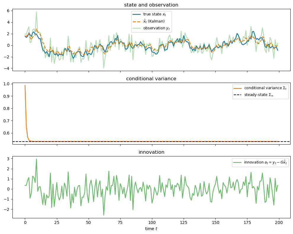
47.9.2. Convergence of the Riccati equation#
The Kalman class computes the steady-state covariance \(\Sigma_\infty\) by
solving the discrete algebraic Riccati equation directly.
Sigma_inf, K_inf = kf.stationary_values()

print(f"Steady-state covariance  Σ_inf = {Sigma_inf[0, 0]:.6f}")
print(f"Kalman filter converged to Σ_t = {Sigmas[-1]:.6f}")
print(f"Steady-state Kalman gain K  = {K_inf[0, 0]:.6f}")

A_minus_KG = A - K_inf @ G
eigval = np.linalg.eigvals(A_minus_KG)[0]
print(f"\nEigenvalue of (A - KG)      = {eigval:.6f}")
print(f"Stable VAR: {np.abs(eigval) < 1}")
Steady-state covariance  Σ_inf = 0.530899
Kalman filter converged to Σ_t = 0.530899
Steady-state Kalman gain K  = 0.312110

Eigenvalue of (A - KG)      = 0.587890
Stable VAR: True
47.9.3. The VAR representation#
Using (47.20), the coefficients in the infinite-order VAR representation are \(G(A - KG)^j K\) for \(j = 0, 1, 2, \ldots\)
We retrieve them via stationary_coefficients:
J = 30
var_coeffs = kf.stationary_coefficients(J, coeff_type='var')

# Lag j+1 coefficient matrices
lags = np.arange(1, J + 1)
coeff_values = np.array([var_coeffs[j][0, 0] for j in range(J)])

fig, ax = plt.subplots()
ax.stem(lags, coeff_values, basefmt=' ')
ax.set_xlabel('lag $j$')
ax.set_ylabel(r'VAR coefficient $G(A{-}KG)^{j-1}K$')
fig.tight_layout()
plt.show()
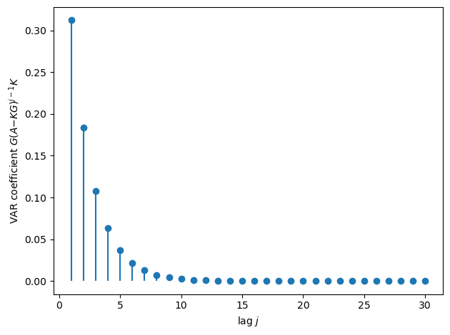
Fig. 47.2 VAR coefficients from the innovations representation#
Most of the autoregressive weight is concentrated in the first few lags.
The later coefficients are nearly zero, so a short finite-lag VAR captures most of the infinite-order representation in this example.
47.9.4. Likelihood evaluation#
We use (47.17) to evaluate the log-likelihood of the simulated sample.
def log_likelihood(A, C, G, R, y_data, x_hat_0, Sigma_0):
    """Evaluate the log-likelihood using the Kalman filter recursions."""
    H_ = np.linalg.cholesky(R)   # R = H_ @ H_.T
    lss_ = qe.LinearStateSpace(A, C, G, H_, mu_0=x_hat_0, Sigma_0=Sigma_0)
    kf_ = qe.Kalman(lss_)
    kf_.set_state(x_hat_0, Sigma_0)

    T_, m_ = y_data.shape
    loglik = 0.0

    for t in range(T_):
        x_h = kf_.x_hat
        Sig = kf_.Sigma
        Omega = G @ Sig @ G.T + R        # innovation covariance
        a_t = y_data[t] - (G @ x_h).flatten()

        sign, logdet = np.linalg.slogdet(Omega)
        loglik += -0.5 * (m_ * np.log(2 * np.pi) + logdet
                          + float(a_t @ np.linalg.solve(Omega, a_t)))
        kf_.update(y_data[t])

    return loglik


y_data_col = y_obs.reshape(-1, 1)
ll = log_likelihood(A, C, G, R,
                    y_data_col,
                    np.zeros(1), np.eye(1) * 10.0)
print(f"Log-likelihood of sample: {ll:.4f}")
Log-likelihood of sample: -325.2335
47.10. An example#
We now work through a structured example that shows how a bivariate VAR(2) fits naturally into the state space framework and how the Kalman filter delivers a Wold (innovations) representation.
47.10.1. A linear state-space system and its filter#
The state and observation equations are
with initial condition and shock distributions
The steady-state error covariance matrix \(\Sigma\) satisfies the Riccati equation
and the associated steady-state Kalman gain is
Starting from an initial estimate \(\hat{x}_0\), the Kalman filter updates the state estimate via
where the innovation is
Substituting (47.32) into (47.31) and expanding:
47.10.2. Impulse responses of \(y_t\) to the innovations \(a_t\)#
It is useful to compute the ordinary impulse response functions of the observable vector \(y_t\) to its own innovations \(a_t\), the moving-average (Wold) representation that is the mirror image of the VAR (47.20).
From the time-invariant innovations representation (47.18)
the moving-average representation (47.25) is
Hence the impulse response of \(y_t\) to a unit innovation \(a_t\) is
These coefficients decay at the rate governed by the eigenvalues of \(A\).
We can read the coefficients (47.34) directly off a quantecon
LinearStateSpace object.
We build a state-space system whose state is the filtered estimate \(\hat{x}_t\), whose single “shock” is the innovation \(a_t\) loaded through \(C = K\), and whose observation matrix is \(G\).
The
impulse_response method of that object returns the sequence \(G A^{j} K\) for
\(j = 0, 1, 2, \ldots\), which are exactly the \(\Psi_h\) for \(h \ge 1\); we prepend
\(\Psi_0 = I\) to capture the contemporaneous feed-through \(y_t = G\hat{x}_t + a_t\).
The array returned below has entry [h, i, j] equal to the response of
observable i at horizon h to innovation component j.
def y_to_a_irf(A, K, G, T=40):
    """
    Return Wold IRFs of y_t to its own innovations a_t.
    """
    n, m = A.shape[0], G.shape[0]
    lss = qe.LinearStateSpace(A, K, G, np.zeros((m, m)), mu_0=np.zeros(n))
    _, ycoef = lss.impulse_response(j=T - 2)      # [GK, GAK, GA^2K, ...]
    Psi = np.empty((T, m, m))
    Psi[0] = np.eye(m)                          # contemporaneous response
    for h in range(1, T):
        Psi[h] = ycoef[h - 1]
    return Psi
47.10.3. Bivariate VAR(2) in state-space form#
Consider two observable series \(r_t\) and \(z_t\).
Stack them into the state vector \(x_t = (r_t,\; r_{t-1},\; z_t,\; z_{t-1})^\top\).
We posit the VAR(2) state-transition equation:
We consider two possible observation equations.
The first is a bivariate observation of \(r_t\) and \(z_t\):
The second is a univariate observation of \(r_t\):
We now compare the Wold impulse responses generated by these two observation systems.
System 1 observes both \(r_t\) and \(z_t\), so its innovation \(a_t\) is \(2 \times 1\).
System 2 observes only \(r_t\), so its innovation \(u_t\) is scalar.
The transition matrices are the same in the two systems, but the observation matrix changes.
Consequently, the steady-state Kalman gain changes too, and so do the Wold responses of the observables to their own innovations.
47.10.4. Numerical example: impulse responses to innovations#
The parameter values are:
These give the \(4 \times 4\) transition matrix and \(4 \times 2\) shock-loading matrix
System 1 uses the bivariate observation equation (47.36), so \(G\) selects \((r_t, z_t)^\top\) from the state and the innovation \(a_t\) is \(2 \times 1\).
System 2 uses the univariate observation equation (47.37), so the row vector in that equation selects only \(r_t\) and the innovation \(u_t\) is scalar.
# Parameters
d1, d2, d3, d4 = 0.80, 0.05, 0.75, -.72
δ1, δ2, δ3, δ4 = 0.00, 0.00, 0.75, 0.20
c11, c12, c21, c22 = 1.0,  0.0,  0.0,  1.0
σ_v = 0.01  # sqrt(0.0001)

# Shared matrices
A_var = np.array([[d1,     d2,     d3,     d4    ],
                  [1.0,    0.0,    0.0,    0.0   ],
                  [δ1, δ2, δ3, δ4],
                  [0.0,    0.0,    1.0,    0.0   ]])

C_var = np.array([[c11, c12],
                  [0.0, 0.0],
                  [c21, c22],
                  [0.0, 0.0]])

# System 1: bivariate observation
G_biv = np.array([[1.0, 0.0, 0.0, 0.0],
                  [0.0, 0.0, 1.0, 0.0]])
H_biv = σ_v * np.eye(2)          # H @ H.T = 0.0001 * I_2

lss_biv = qe.LinearStateSpace(A_var, C_var, G_biv, H_biv,
                               mu_0=np.zeros(4), Sigma_0=np.eye(4))
kf_biv = qe.Kalman(lss_biv)
_, K_biv = kf_biv.stationary_values()

print("System 1 - steady-state Kalman gain K (4x2):")
print(np.round(K_biv, 5))

# System 2: univariate observation
G_uni = np.array([[1.0, 0.0, 0.0, 0.0]])
H_uni = np.array([[σ_v]])         # H @ H.T = 0.0001

lss_uni = qe.LinearStateSpace(A_var, C_var, G_uni, H_uni,
                               mu_0=np.zeros(4), Sigma_0=np.eye(4))
kf_uni = qe.Kalman(lss_uni)
_, K_uni = kf_uni.stationary_values()

print("\nSystem 2 - steady-state Kalman gain K (4x1):")
print(np.round(K_uni, 5))
System 1 - steady-state Kalman gain K (4x2):
[[7.9987e-01 7.4987e-01]
 [9.9990e-01 0.0000e+00]
 [1.0000e-05 7.4994e-01]
 [0.0000e+00 9.9990e-01]]

System 2 - steady-state Kalman gain K (4x1):
[[0.72306]
 [0.99994]
 [0.31829]
 [0.30984]]
We now apply the helper y_to_a_irf defined above to compute the ordinary
impulse responses (47.34) of the observable \(y_t\) to its own
innovations \(a_t\), for both System 1 (bivariate, so \(a_t\) is \(2 \times 1\)) and
System 2 (univariate, so \(u_t\) is scalar).
T_irf = 40
horizons = np.arange(T_irf)

Psi_biv = y_to_a_irf(A_var, K_biv, G_biv, T_irf)   # System 1: (T, 2, 2)
Psi_uni = y_to_a_irf(A_var, K_uni, G_uni, T_irf)   # System 2: (T, 1, 1)

obs_labels = [r'$r_t$', r'$z_t$']
innov_labels = [r'$a_{1,t}$', r'$a_{2,t}$']

# System 1 responses
fig, axes = plt.subplots(2, 2, figsize=(10, 6), sharex=True)
for i, obs in enumerate(obs_labels):
    for j, inn in enumerate(innov_labels):
        ax = axes[i, j]
        ax.plot(horizons, Psi_biv[:, i, j], lw=2)
        ax.axhline(0, color='k', lw=0.6, ls='--')
        ax.set_title(fr'{obs} to {inn}', fontsize=9)
        if i == 1:
            ax.set_xlabel('horizon $h$')
        if j == 0:
            ax.set_ylabel('response')
fig.tight_layout()
plt.show()
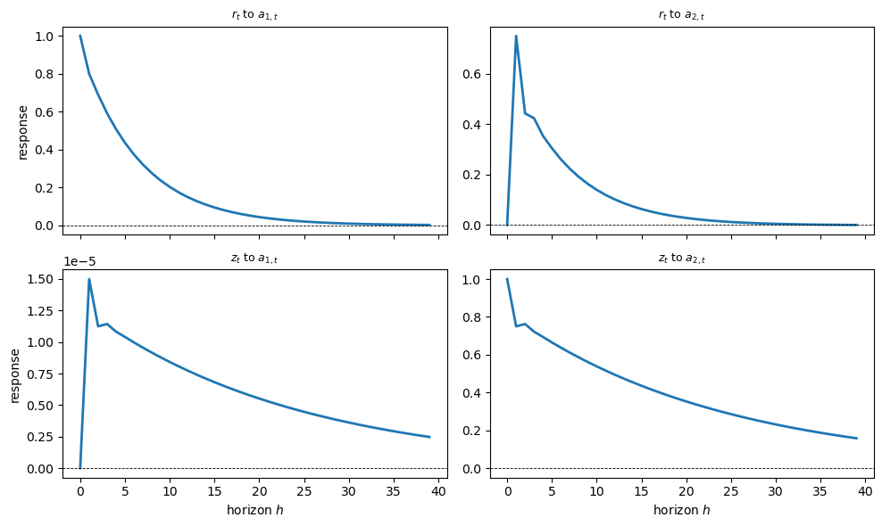
Fig. 47.3 System 1 responses to own innovations#
Own innovations move their own observables one-for-one on impact and then fade.
The diagonal panels start at one and the off-diagonal panels start at zero because \(\Psi_0 = I\).
The cross response of \(r_t\) to \(a_{2,t}\) is sizeable at short horizons, while the response of \(z_t\) to \(a_{1,t}\) is tiny on the displayed scale.
fig, ax = plt.subplots()
ax.plot(horizons, Psi_uni[:, 0, 0], lw=2)
ax.axhline(0, color='k', lw=0.6, ls='--')
ax.set_xlabel('horizon $h$')
ax.set_ylabel('response')
fig.tight_layout()
plt.show()
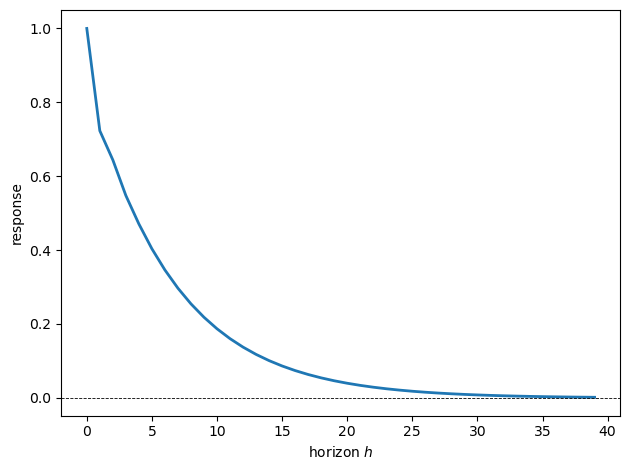
Fig. 47.4 System 2 response to own innovation#
With only \(r_t\) observed, the single innovation moves \(r_t\) one-for-one on impact and then decays monotonically toward zero.
For \(h \ge 1\) the responses propagate through the state matrix \(A\) and decay geometrically, tracing out the Wold moving-average representation of the bivariate (System 1) and univariate (System 2) processes.
These are forecast-error responses from the Wold representation, not structural shock responses.
With the example in place, we can now pull together the main lessons of the lecture.
47.11. Summary#
The Kalman filter recursively updates beliefs about a hidden state by combining a prior forecast with the new information contained in the current observation.
The Riccati equation tracks how the filter’s conditional covariance evolves, and its steady state makes the filter time invariant.
At that steady state, the innovations representation writes the observable process in terms of one-step forecast errors that are white noise by construction.
Solving the innovations representation backward gives an infinite-order VAR, while solving it forward gives the Wold moving-average representation.
The numerical examples show that changing the observed variables changes the Kalman gain and therefore changes the Wold responses, even when the underlying state dynamics are the same.
47.12. Exercises#
Exercise 47.1
Consider the scalar AR(1) state space system used above with \(\rho = 0.9\), \(\sigma_w = 0.5\), \(\sigma_v = 1.0\).
Derive an algebraic expression for the steady-state conditional variance \(\Sigma_\infty\) by solving the scalar Riccati equation (47.14) at its fixed point \(\Sigma_{t+1} = \Sigma_t = \Sigma\).
Show that \(\Sigma\) satisfies a quadratic equation, find its positive root, and
verify numerically that your formula matches kf.Sigma_infinity.
Solution
Here is one solution:
Setting \(\Sigma_{t+1} = \Sigma_t = \Sigma\) in the scalar version of (47.14) with \(A = \rho\), \(CC^\top = \sigma_w^2\), \(GG^\top = 1\), \(R = \sigma_v^2\):
Multiplying through by \(\Sigma + \sigma_v^2\) and rearranging:
Taking the positive root of this quadratic:
ρ_, σ_w_, σ_v_ = 0.9, 0.5, 1.0

b = σ_v_**2 * (1 - ρ_**2) - σ_w_**2
discriminant = b**2 + 4 * σ_v_**2 * σ_w_**2
Sigma_formula = (-b + np.sqrt(discriminant)) / 2

A_ = np.array([[ρ_]])
C_ = np.array([[σ_w_]])
G_ = np.array([[1.0]])
R_ = np.array([[σ_v_**2]])
H_ = np.array([[σ_v_]])   # R_ = H_ @ H_.T
lss_ = qe.LinearStateSpace(A_, C_, G_, H_, mu_0=np.zeros(1), Sigma_0=np.eye(1))
kf_ = qe.Kalman(lss_)

print(f"Analytical Σ_inf   = {Sigma_formula:.8f}")
print(f"Numerical  Σ_inf   = {kf_.Sigma_infinity[0, 0]:.8f}")
Analytical Σ_inf   = 0.53089919
Numerical  Σ_inf   = 0.53089919
Exercise 47.2
This exercise considers a two-dimensional state with a one-dimensional observation:
Simulate \(T = 500\) observations from this system starting from a diffuse prior.
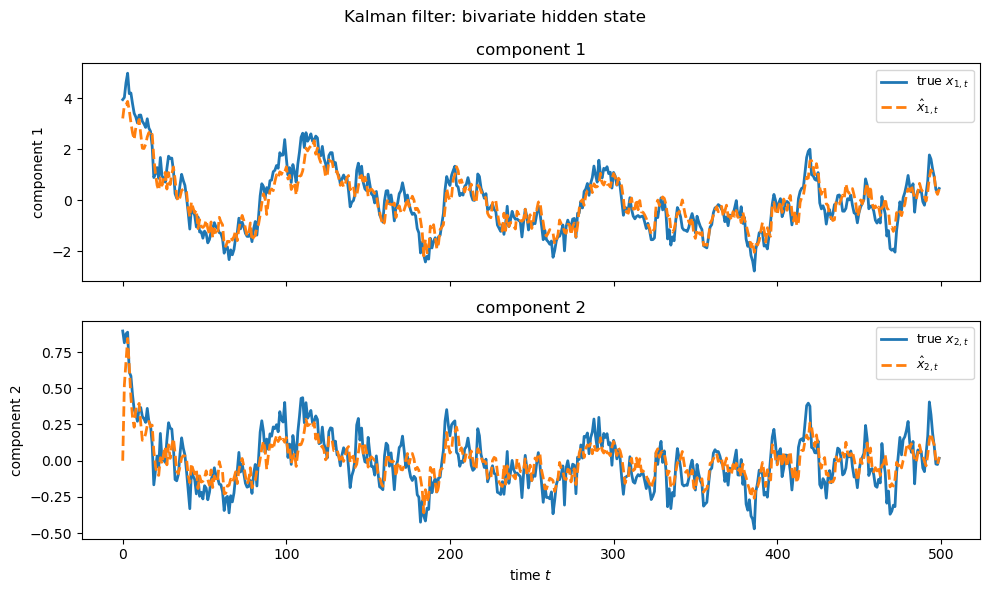
Run the Kalman filter and plot both components of \(\hat{x}_t\) against the true hidden state path.
Compute and report the steady-state covariance \(\Sigma_\infty\) and Kalman gain \(K_\infty\).
Check that the eigenvalues of \(A - K_\infty G\) lie strictly inside the unit circle, confirming that the VAR representation (47.20) is stable.
Solution
Here is one solution:
A2 = np.array([[0.9, 0.1],
               [0.0, 0.8]])
C2 = np.array([[0.4],
               [0.1]])
G2 = np.array([[1.0, 0.0]])
R2 = np.array([[0.5]])
H2 = np.array([[np.sqrt(0.5)]])   # R2 = H2 @ H2.T

lss2 = qe.LinearStateSpace(A2, C2, G2, H2,
                             mu_0=np.zeros(2),
                             Sigma_0=np.eye(2) * 5.0)
kf2 = qe.Kalman(lss2)
kf2.set_state(np.zeros(2), np.eye(2) * 5.0)

T2 = 500
x2_path, y2_path = lss2.simulate(ts_length=T2, random_state=0)

x_hats2 = np.zeros((T2, 2))
for t in range(T2):
    kf2.update(y2_path[:, t])
    x_hats2[t] = kf2.x_hat.ravel()

fig, axes = plt.subplots(2, 1, figsize=(10, 6), sharex=True)
for i, ax in enumerate(axes):
    ax.plot(x2_path[i, :T2], lw=2, label=f'true $x_{{{i+1},t}}$')
    ax.plot(x_hats2[:, i], lw=2, ls='--', label=rf'$\hat{{x}}_{{{i+1},t}}$')
    ax.set_title(f'component {i+1}')
    ax.legend(fontsize=9)
    ax.set_ylabel(f'component {i+1}')
axes[1].set_xlabel('time $t$')
fig.suptitle('Kalman filter: bivariate hidden state')
fig.tight_layout()
plt.show()

# Steady-state values
Sigma2_inf, K2_inf = kf2.stationary_values()
print("Steady-state covariance Σ_inf:")
print(np.round(Sigma2_inf, 5))
print("\nSteady-state Kalman gain K_inf:")
print(np.round(K2_inf, 5))

# Eigenvalues of A - K_inf G
AKG2 = A2 - K2_inf @ G2
eigvals2 = np.linalg.eigvals(AKG2)
print(f"\nEigenvalues of A - K_inf G: {np.round(eigvals2, 5)}")
print(f"Stable VAR: {np.all(np.abs(eigvals2) < 1)}")
Steady-state covariance Σ_inf:
[[0.32854 0.07219]
 [0.07219 0.0166 ]]

Steady-state Kalman gain K_inf:
[[0.36559]
 [0.06971]]

Eigenvalues of A - K_inf G: [0.56394 0.77047]
Stable VAR: True
After the diffuse-prior transient, both Kalman estimates move closely with their corresponding hidden state paths.
The second component is not observed directly, so its tracking comes from the state dynamics and its connection to the observed signal.
The printed eigenvalues then check the separate stability condition for the VAR representation.
Exercise 47.3
This exercise studies likelihood and parameter estimation using the scalar model from the main text with true parameters \((\rho, \sigma_w, \sigma_v) = (0.9, 0.5, 1.0)\):
Simulate \(T = 300\) observations.
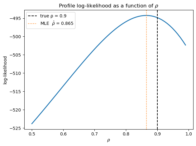
Write a function that evaluates the log-likelihood as a function of \(\rho \in (0, 1)\), holding \(\sigma_w = 0.5\) and \(\sigma_v = 1.0\) fixed, and plot the log-likelihood against \(\rho\) for a grid of values.
Locate the maximum numerically and check that it is close to the true value \(\rho = 0.9\).
Solution
Here is one solution:
# True parameters
ρ_true, sw_true, sv_true = 0.9, 0.5, 1.0

A_t = np.array([[ρ_true]])
C_t = np.array([[sw_true]])
G_t = np.array([[1.0]])
R_t = np.array([[sv_true**2]])
H_t = np.array([[sv_true]])   # R_t = H_t @ H_t.T

lss_t = qe.LinearStateSpace(A_t, C_t, G_t, H_t,
                             mu_0=np.zeros(1), Sigma_0=np.eye(1))
_, y_sim = lss_t.simulate(ts_length=300, random_state=7)
y_sim = y_sim.T          # shape (300, 1)

def ll_rho(ρ_val):
    A_ = np.array([[ρ_val]])
    C_ = np.array([[sw_true]])
    G_ = np.array([[1.0]])
    R_ = np.array([[sv_true**2]])
    return log_likelihood(A_, C_, G_, R_, y_sim,
                          np.zeros(1), np.eye(1) * 10.0)

ρ_grid = np.linspace(0.5, 0.99, 60)
ll_vals = np.array([ll_rho(r) for r in ρ_grid])

ρ_mle = ρ_grid[np.argmax(ll_vals)]

fig, ax = plt.subplots()
ax.plot(ρ_grid, ll_vals, lw=2)
ax.axvline(ρ_true, color='k',   ls='--', label=f'true ρ = {ρ_true}')
ax.axvline(ρ_mle, color='C1', ls=':', label=f'MLE  $\\hat{{\\rho}}$ = {ρ_mle:.3f}')
ax.set_xlabel(r'$\rho$')
ax.set_ylabel('log-likelihood')
ax.set_title('Profile log-likelihood as a function of $\\rho$')
ax.legend()
fig.tight_layout()
plt.show()

print(f"True ρ = {ρ_true},  MLE ρ_hat = {ρ_mle:.4f}")
True ρ = 0.9, MLE ρ_hat = 0.8654
The likelihood curve is single-peaked and reaches its maximum close to the true value \(\rho = 0.9\).
The small gap between the grid maximizer and the true value comes from finite-sample randomness and the use of a discrete grid.